Open Access
Research Article
Max Screen >>
ISSN: 2348-9790
Copyright: © 2014 Parés-Casanova PM. This is an open-access article distributed under the terms of the Creative Commons Attribution License, which permits unrestricted use, distribution, and reproduction in any medium, provided the original author and source are credited.
Related article at Pubmed, Google Scholar
This study involved some morphometric parameters of the skull of thirty adult Gwembe Dwarf Goats (15 males and 15 females) without any apparent skeletal disorders. Lower jaws were not included in this study. A total of 43 linear measurements were analyzed. The analysis reflected no differences between sexes, thereby indicating lack of general conformation differences between males and females. However, comparison of the parameters that exhibited most variance revealed that horncore basal circumference and length of the horn core on the front margin were strongly influenced by sex. Therefore, only the horn conformation could be used as discriminator sexual variable. This result couples with the fact that males usually have stronger and larger horns than females but skull size seeming no to be very different between sexes. The obtained results would indicate a marked sexual monomorphism in this breed.
Keywords: Capra hircus; Craniometry; Sexual dimorphism; Skull biometryMaterials
Local goat has great genetic resource potential that can be utilized as a source of superior breeding formulation adaptable to local conditions. [1] Reported that breeds of local livestock are important and should be protected because of their ability to survive under low-quality feed, unfavourable local climatic conditions, and their high resistance to local diseases and parasites. These abilities are critical in cross-breeding ventures aimed at sustaining genetic pools that have evolved through centuries within the given locality.
Phenotypic and morphological characteristics are still commonly used by researchers and practitioners in characterization of animals' breeds [2]. The Gwembe Dwarf Goat or locally known as "Mpongo" is a small breed with average weight of 35 kg for both males and females found in the Gwembe valley in Southern Province of Zambia. Well-adapted to hot and dry climatic conditions with low rainfall patterns, this breed is of multi colour coat variations ranging from completely black, brown, black and white, grey to white and brown- with horns of medium size and usually curved backwards (https://dad.fao.org/). Other goat breeds of Zambia include the Plateau Goat located on the plateau regions of Southern Province, the Sinazongwe district of the Southern and North part of the Gwembe Valley, and the imported Boer and Saanen (https://dad.fao.org/). The morphologic and morphometric studies of the head region do not only reflect contributions of genetic and environmental components to individual development, but describe genetic and ecophenotypic variation [3]. Until now, there have been numerous comparative morphological studies of the skull anatomy in many of the mammalian species. In particular, in small ruminants the morphological structures and geometrical measurements of the skull bones have been examined to detect the distinguishing features of these species [4] and breeds [3,5,6]. To the best knowledge of the authors, there is no published data on the morphometric parameters of the head region applied anatomy in the Zambian native goats. An exception of this is the thesis by [7], which does not contain detailed information on head conformation other than the head length and width for male and female goats of unknown breed. Moreover, complete comparative studies between sexes are not available.
So, the morphometric values of the skull of the Gwembe Dwarf Goat will not only be of ethnological importance but they will undoubtedly aid to better the description of sexual differences. Furthermore, the obtained results will provide important baseline data for further comparative studies on the skull of the Zambian native goat breeds.
Thirty dry skulls of adult Gwembe Dwarf Goat specimens aged 18 months and older were collected from five different local farms and studied. The age was determined on the basis of the growth of the third molar tooth [8]. All specimens used for this study showed no cranial deformities or bony injuries. The total series included all specimens collected.
The method described by [9] was used for assessing cranial (neuro- and viscerocranium) linear measurements, and it is commonly used in other osteometric studies [10]. A total of 43 linear measurements were analyzed (Table 1). Lower jaws were not included in this study. Basic descriptive statistics were calculated for all samples and no size adjustment was applied. The measurements were performed using 0.1 mm callipers and an ovinometer. All measurements were taken by the same person (Kataba).
Main simple descriptive statistics (range, mean, standard deviation and coefficient of variation) were obtained, as well the to assess normality of distribution of data in both sexes. The non-parametric one-way NPMANOVA test (Non-Parametric MANOVA, also known as PERMANOVA) was applied, using the Mahalanobis distance [11]. The significance was computed by permutation of group membership, with 9,999 replicates. Given the large number of parameters, a selection of the most relevant parameters was ultimately made using a multivariate analysis of principal components (PCA). The principal components (PC) were extracted from the co-variance matrix. The eigenanalysis was carried out on the group means ("between-group", i.e. the items analysed are the groups, not the specimens). The loadings within the individual eigenvectors for each PC were used to form contrasts in order to describe the skulls numerically. A one-way MANOVA (Multivariate ANalysis Of VAriance) tested whether male and female samples had the same mean for the most discriminant parameters. The two-sample Hotelling's T2 test was avoided as some of these parameter were non parametric. In order to identify and measure the associations among the two sets of parameters, a Canonical Correspondence Analysis was done, according to [12] and the two-tailed non-parametric U Mann-Whitney was used to test whether the medians of samples (males and females) were different.
The data recorded were analyzed statistically in customary fashion using PAST® (v. 2.17c) software. Level confidence was stablished at 5%.
In Table 2 there appear the main descriptive statistics for linear measurements. The NPMANOVA reflected no differences between sexes (F=1.104, p=0.317), so it can be supposed that there appeared no general conformation differences between males and females.
For the PCA, first 6 PCs presented a eigenvalue higher of Jollife cut-off's one (0.363). PC1 explained a 43% of variance (Table 3). The most important parameters that entered into the PC1 were 40 (horncore basal circumference) and 43 (length of the horn core on the front margin), both related to horns, and into the PC2 was 40. For PC3 was the parameter 4 (short skull length), which presented the highest value (Table 4). For these parameters, NPMANOVA did reflect differences between sexes (F=4.752, p=0.006), so sexual dimorphism can be suspected not for a general skull form but only for horns. Horn parameters that had strong influence on the sex were precisely the length of the horn core on the front margin (1.239, Can1) and the horncore basal circumference (-0.935, Can1) (Figure 1), the latter one (but not the former) (U=65.5, p=0.053) being statistically different between sexes (U=20.5, p<0.001) (Figure 2).
Dimorphism means two forms "sexual dimorphism" means that the two sexes of a species differ in external appearance or other features. Males and females may differ in size, color, shape, the development of appendages (such as horns, teeth, feathers, or fins), and also in scent or sound production. Species in which male and females are identical in appearance or other features are said to be "monomorphic". Our results showed that there are no general skull conformation differences between males and females in the Dwarf Zambian Goat, although some particular parameters have an strong influence on the breed sex, such as the length of the horn core on the front margin, the distance between horn tips, and the short skull length. This is in line with the fact that males usually have stronger and larger horns than females [8]. Short skull length (parameter 4) has low influence, so size seems not to be very different between sexes. According to [7] 2009, males and females would differ by their head width, not by their head length, but, as earlier stated, his research is not clearly focused on Dwarf goat.
The global variation between sexes may be interpreted in relation to extensive management styles of the animals that are moreover under a low anthropogenic influence so they tend to reinforce the natural sexual size dimorphism of the species. Thus, horn conformation could be used as discriminator sexual variable and this fact can be attributed to that sexual dimorphism in this breed is not related to differences in the diet of the two sexes but probably to participation in fighting between males, or to a mere artificial selection of males towards bigger horns by farmers.

![]()

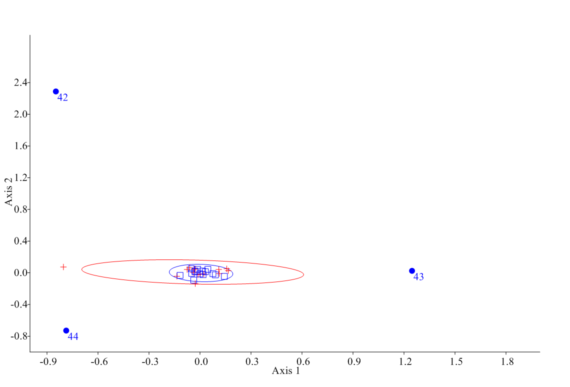 |
| Figure 1: Canonical Analysis for horn parameters (95% confidence ellipses), showing the position of individuals according to their horn conformation (squares for males, n=15, crosses for females, n=15). Number on dots show each analyzed parameter (42: least diameter of horn core base; 43: length of the horn core on the front margin; 44: distance between horn tips). |
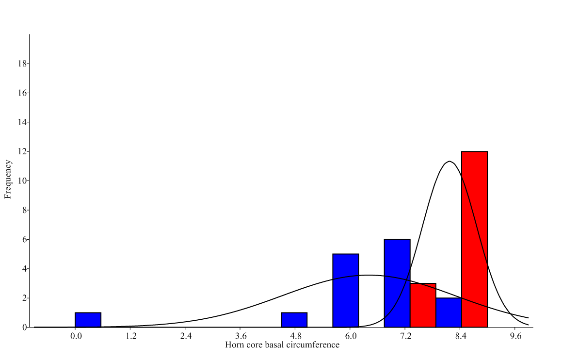 |
| Figure 2: Histogram of horncores basal circumferences for males (right, n=15) and females (left, n=15). This parameter that shows statistically differences between sexes (Mann-Whitney's U=20.5, p<0.001). |
| Parameter | Definition |
|---|---|
| 1 | Total length of the skull: the distance between akrokranion-prosthion |
| 2 | Condylobasal length: caudal border of occipital condyles-prosthion |
| 3 | Total length of the cranial base: basion-prosthion |
| 4 | Short skull length: basion-premolare |
| 5 | Premolare-prosthion length |
| 7 | Upper length of the viscerocranium: nasion-prosthion |
| 8 | Median frontal length: akrokranion-nasion |
| 9 | Akrokranion-bregma length |
| 10 | Frontal length: bregma-nasion |
| 11 | Upper neurocranium length: akrokranion-supraorbitale |
| 12 | Facial length: supraorbitale-prosthion |
| 13 | Akrokranion-infraorbitale length |
| 14 | Greatest length of the lacrimal bone: most lateral point of the lacrimal bone –most rostral point of the lacrimomaxillary suture |
| 15 | Greatest length of the nasal bone: nasion-rhinion |
| 16 | Entorbitale-prosthion length |
| 17 | Distance between the caudal border of one occipital condyle and the infraorbitale of the same side |
| 18 | Dental length: postdentale-prosthion |
| 19 | Oral palatal length: palatinoorale-prosthion |
| 20 | Lateral length of the premaxilla: nasointermaxillare-prosthion |
| 21 | Length of the maxillary tooth row |
| 22 | Length of the upper molar row |
| 23 | Length of the upper premolar row |
| 24 | Greatest inner width of the orbit: ectorbitale-entorbitale |
| 25 | Greatest inner height of the orbit |
| 26 | Greatest mastoid breadth: otion-otion |
| 27 | Greatest breadth of the occipital condyles |
| 28 | Greatest breadth at the bases of the paracondylar processes |
| 29 | Greatest breadth of the foramen magnum |
| 30 | Height of the foramen magnum: basion-opisthion |
| 31 | Least breadth of parietal |
| 32 | Greatest breadth between the lateral borders of horn core base |
| 33 | Greatest neurocranium breadth: euryon-euryon |
| 34 | Greatest frontal breadth: ectorbitale-ectorbitale |
| 35 | Least breadth between the orbits: entorbitale-entorbitale |
| 36 | Facial breadth: between facial tuberosities |
| 37 | Greatest breadth across the nasal bones |
| 38 | Greatest breadth across the premaxilla |
| 39 | Greatest palatal breadth |
| 40 | Horncore basal circumference |
| 41 | Greatest diameter of horn core base |
| 42 | Least diameter of horn core base |
| 43 | Length of the horn core on the front margin |
| 44 | Distance between horn tips |
| Table 1: Studied parameters (nomenclature according to Von den Driesch, 1976). A total of 43 linear measurements were analyzed. Von den Driesch's numeration has been served, except for var. 44 which is ours. | |
| ♀ | ♂ | |||||||||||||
|---|---|---|---|---|---|---|---|---|---|---|---|---|---|---|
| Var. | Min | Max | X | StD | CV | W | P | Min | Max | X | StD | CV | W | P |
| 1 | 13.0 | 16.7 | 15.1 | 1.319 | 8.7 | 0.908 | 0.125 | 13.4 | 16.7 | 15.0 | 0.858 | 5.7 | 0.944 | 0.438 |
| 2 | 12.6 | 16.4 | 14.3 | 1.389 | 9.7 | 0.897 | 0.085 | 12.5 | 15.8 | 14.7 | 0.746 | 5.1 | 0.801 | 0.004 |
| 3 | 11.8 | 14.5 | 13.1 | 0.786 | 6.0 | 0.969 | 0.839 | 11.6 | 14.1 | 12.6 | 0.757 | 6.0 | 0.953 | 0.573 |
| 4 | 7.7 | 10.3 | 9.1 | 0.789 | 8.7 | 0.963 | 0.742 | 7.5 | 10.3 | 8.2 | 0.685 | 8.3 | 0.783 | 0.002 |
| 5 | 3.5 | 4.6 | 4.0 | 0.348 | 8.6 | 0.956 | 0.622 | 3.5 | 4.3 | 4.0 | 0.254 | 6.4 | 0.951 | 0.541 |
| 7 | 7.8 | 9.8 | 8.6 | 0.669 | 7.8 | 0.921 | 0.198 | 7.5 | 9.4 | 8.5 | 0.534 | 6.3 | 0.974 | 0.917 |
| 8 | 7.7 | 10.0 | 9.1 | 0.680 | 7.5 | 0.946 | 0.464 | 7.8 | 9.8 | 8.6 | 0.536 | 6.2 | 0.939 | 0.365 |
| 9 | 4.6 | 5.3 | 5.0 | 0.197 | 3.9 | 0.951 | 0.533 | 4.3 | 5.2 | 4.9 | 0.246 | 5.0 | 0.924 | 0.218 |
| 10 | 5.3 | 6.4 | 5.9 | 0.340 | 5.8 | 0.967 | 0.815 | 5.3 | 6.6 | 6.0 | 0.369 | 6.1 | 0.947 | 0.484 |
| 11 | 8.2 | 9.3 | 8.9 | 0.342 | 3.8 | 0.888 | 0.063 | 8.0 | 10.0 | 9.1 | 0.711 | 7.8 | 0.928 | 0.251 |
| 12 | 9.0 | 10.6 | 9.8 | 0.403 | 4.1 | 0.981 | 0.976 | 8.4 | 10.3 | 9.5 | 0.563 | 5.9 | 0.93 | 0.269 |
| 13 | 9.9 | 12.0 | 10.6 | 0.615 | 5.8 | 0.923 | 0.213 | 10.0 | 11.5 | 10.7 | 0.443 | 4.1 | 0.931 | 0.285 |
| 14 | 1.9 | 3.3 | 2.6 | 0.369 | 14.2 | 0.991 | 1.000 | 2.0 | 2.9 | 2.6 | 0.218 | 8.5 | 0.948 | 0.491 |
| 15 | 3.9 | 5.6 | 4.8 | 0.556 | 11.7 | 0.943 | 0.422 | 4.0 | 5.5 | 4.6 | 0.411 | 9.0 | 0.889 | 0.065 |
| 16 | 7.5 | 9.9 | 8.8 | 0.739 | 8.4 | 0.966 | 0.791 | 7.7 | 9.7 | 8.9 | 0.578 | 6.5 | 0.959 | 0.671 |
| 17 | 10.1 | 11.9 | 11.0 | 0.658 | 6.0 | 0.928 | 0.251 | 9.9 | 11.8 | 11.1 | 0.525 | 4.7 | 0.94 | 0.383 |
| 18 | 6.9 | 8.7 | 7.9 | 0.588 | 7.4 | 0.923 | 0.212 | 6.6 | 8.5 | 7.6 | 0.467 | 6.1 | 0.981 | 0.976 |
| 19 | 5.7 | 6.8 | 6.2 | 0.371 | 5.9 | 0.854 | 0.020 | 5.1 | 6.5 | 6.0 | 0.377 | 6.3 | 0.947 | 0.484 |
| 20 | 5.1 | 6.3 | 5.6 | 0.439 | 7.8 | 0.849 | 0.017 | 4.7 | 6.0 | 5.5 | 0.401 | 7.3 | 0.936 | 0.333 |
| 21 | 4.3 | 5.6 | 5.0 | 0.449 | 9.0 | 0.918 | 0.180 | 4.1 | 5.3 | 4.6 | 0.388 | 8.5 | 0.887 | 0.060 |
| 22 | 2.5 | 3.1 | 2.8 | 0.149 | 5.2 | 0.926 | 0.237 | 2.6 | 2.9 | 2.8 | 0.097 | 3.5 | 0.903 | 0.107 |
| 23 | 1.5 | 2.7 | 2.2 | 0.443 | 20.5 | 0.873 | 0.038 | 1.4 | 2.5 | 1.9 | 0.403 | 20.7 | 0.887 | 0.060 |
| 24 | 2.8 | 3.3 | 3.1 | 0.171 | 5.5 | 0.952 | 0.556 | 2.8 | 3.4 | 3.1 | 0.188 | 6.0 | 0.934 | 0.314 |
| 25 | 2.9 | 3.2 | 3.1 | 0.093 | 3.0 | 0.944 | 0.429 | 2.8 | 3.4 | 3.2 | 0.167 | 5.3 | 0.981 | 0.973 |
| 26 | 5.4 | 6.2 | 5.9 | 0.223 | 3.8 | 0.884 | 0.055 | 5.2 | 6.2 | 5.8 | 0.308 | 5.3 | 0.924 | 0.218 |
| 27 | 3.8 | 4.4 | 4.1 | 0.168 | 4.1 | 0.942 | 0.402 | 4.0 | 4.3 | 4.1 | 0.087 | 2.1 | 0.92 | 0.192 |
| 28 | 4.8 | 5.9 | 5.3 | 0.251 | 4.7 | 0.954 | 0.589 | 5.0 | 5.7 | 5.3 | 0.177 | 3.3 | 0.95 | 0.522 |
| 29 | 1.6 | 2.0 | 1.9 | 0.106 | 5.7 | 0.973 | 0.897 | 1.5 | 2.0 | 1.8 | 0.136 | 7.5 | 0.913 | 0.151 |
| 30 | 1.5 | 1.8 | 1.6 | 0.093 | 5.7 | 0.93 | 0.269 | 1.4 | 1.7 | 1.6 | 0.105 | 6.6 | 0.936 | 0.331 |
| 31 | 2.2 | 3.9 | 2.9 | 0.430 | 14.7 | 0.952 | 0.556 | 2.7 | 3.7 | 3.1 | 0.318 | 10.1 | 0.946 | 0.461 |
| 32 | 5.5 | 7.2 | 6.4 | 0.416 | 6.5 | 0.981 | 0.976 | 6.2 | 7.1 | 6.8 | 0.276 | 4.1 | 0.928 | 0.256 |
| 33 | 5.6 | 6.6 | 5.9 | 0.264 | 4.5 | 0.795 | 0.003 | 5.4 | 6.0 | 5.8 | 0.191 | 3.3 | 0.95 | 0.524 |
| 34 | 7.3 | 9.1 | 8.2 | 0.485 | 5.9 | 0.936 | 0.331 | 7.6 | 8.5 | 8.1 | 0.283 | 3.5 | 0.942 | 0.413 |
| 35 | 5.4 | 7.3 | 6.4 | 0.479 | 7.5 | 0.975 | 0.922 | 5.7 | 6.9 | 6.3 | 0.272 | 4.3 | 0.949 | 0.511 |
| 36 | 5.0 | 6.1 | 5.6 | 0.333 | 5.9 | 0.938 | 0.357 | 5.1 | 6.0 | 5.6 | 0.244 | 4.4 | 0.982 | 0.979 |
| 37 | 1.6 | 2.5 | 2.1 | 0.237 | 11.1 | 0.983 | 0.984 | 1.7 | 2.4 | 2.1 | 0.232 | 11.2 | 0.944 | 0.433 |
| 38 | 1.7 | 2.3 | 2.1 | 0.189 | 9.0 | 0.905 | 0.112 | 1.7 | 2.3 | 2.1 | 0.151 | 7.1 | 0.961 | 0.716 |
| 39 | 5.0 | 5.9 | 5.5 | 0.275 | 5.0 | 0.963 | 0.747 | 5.0 | 5.9 | 5.4 | 0.246 | 4.5 | 0.979 | 0.959 |
| 40 | 0.0 | 8.0 | 6.4 | 1.954 | 30.5 | 0.672 | 0.000 | 6.8 | 9.0 | 8.2 | 0.615 | 7.5 | 0.94 | 0.382 |
| 41 | 1.8 | 2.9 | 2.4 | 0.328 | 13.8 | 0.962 | 0.732 | 2.2 | 3.2 | 2.8 | 0.260 | 9.3 | 0.982 | 0.982 |
| 42 | 1.5 | 2.1 | 1.9 | 0.208 | 11.2 | 0.897 | 0.085 | 1.9 | 2.5 | 2.1 | 0.169 | 7.9 | 0.905 | 0.114 |
| 43 | 0.0 | 6.8 | 4.9 | 1.611 | 33.1 | 0.817 | 0.006 | 4.5 | 8.4 | 6.0 | 1.089 | 18.2 | 0.928 | 0.251 |
| 44 | 4.5 | 7.9 | 5.9 | 0.939 | 15.9 | 0.968 | 0.930 | 6.0 | 8.9 | 7.0 | 0.748 | 10.7 | 0.881 | 0.048 |
| X: average StD: Standard Deviation CV: Coefficient of Variation (%) W: Shapiro-Wilk Table 2: Main descriptive statistics for linear measurements (expressed in mm) for females (♀, n=15) and males (♂, n=15). Von den Driesch's numeration has been served, except for var. 44 which is ours. Not normally distributed data appear in bold. |
||||||||||||||
| Pc | Eigenvalue | % variance | % total explained |
|---|---|---|---|
| 1 | 6.486 | 43.042 | 43.042 |
| 2 | 3.422 | 22.705 | 65.747 |
| 3 | 1.369 | 9.085 | 74.832 |
| 4 | 0.925 | 6.141 | 80.973 |
| 5 | 0.691 | 4.586 | 85.559 |
| 6 | 0.390 | 2.589 | 88.148 |
| Table 3: Eigenvalues and % variances for first 6 Principal Components (PCs). Jollife cut-off=0.363. | |||
| PC1 | PC2 | PC3 | |
|---|---|---|---|
| 1 | 0.263 | 0.359 | -0.330 |
| 2 | 0.337 | 0.282 | -0.325 |
| 3 | 0.110 | 0.295 | 0.335 |
| 4 | 0.012 | 0.281 | 0.498 |
| 5 | 0.048 | 0.108 | -0.080 |
| 7 | 0.106 | 0.143 | 0.161 |
| 8 | -0.051 | 0.133 | 0.331 |
| 9 | 0.018 | 0.033 | 0.034 |
| 10 | 0.064 | 0.034 | -0.092 |
| 11 | 0.042 | -0.056 | 0.301 |
| 12 | 0.061 | 0.111 | 0.171 |
| 13 | 0.145 | 0.091 | -0.097 |
| 14 | 0.064 | 0.090 | 0.007 |
| 15 | 0.093 | 0.127 | 0.005 |
| 16 | 0.144 | 0.153 | -0.189 |
| 17 | 0.181 | 0.116 | 0.031 |
| 18 | 0.124 | 0.214 | 0.027 |
| 19 | 0.069 | 0.164 | 0.013 |
| 20 | 0.094 | 0.121 | 0.038 |
| 21 | 0.062 | 0.142 | 0.091 |
| 22 | -0.001 | 0.027 | -0.002 |
| 23 | 0.062 | 0.112 | 0.004 |
| 24 | 0.033 | 0.040 | -0.065 |
| 25 | 0.015 | -0.004 | 0.069 |
| 26 | 0.023 | 0.061 | 0.027 |
| 27 | 0.013 | -0.002 | -0.010 |
| 28 | 0.035 | 0.051 | -0.001 |
| 29 | -0.016 | 0.002 | -0.002 |
| 30 | -0.017 | 0.002 | -0.011 |
| 31 | -0.043 | -0.098 | -0.131 |
| 32 | 0.090 | -0.050 | 0.032 |
| 33 | 0.023 | 0.038 | -0.031 |
| 34 | 0.045 | 0.130 | 0.011 |
| 35 | 0.082 | 0.125 | 0.049 |
| 36 | 0.057 | 0.094 | -0.004 |
| 37 | 0.013 | 0.039 | 0.037 |
| 38 | 0.025 | 0.025 | 0.003 |
| 39 | 0.055 | 0.083 | 0.053 |
| 40 | 0.541 | -0.439 | 0.091 |
| 41 | 0.072 | -0.113 | 0.132 |
| 42 | 0.043 | -0.047 | -0.038 |
| 43 | 0.506 | -0.252 | 0.092 |
| 44 | 0.264 | -0.161 | 0.159 |
| Table 4: Component loading for each parameter for first 3 Principal Component (PC), which explained the 75% of the total observed variance. Highest absolute values for each component appear in bold. | |||