Open Access
Short Communication
Max Screen >>
ISSN: 2455-7625
Copyright: © 2014 Upton G. This is an open-access article distributed under the terms of the Creative Commons Attribution License, which permits unrestricted use, distribution, and reproduction in any medium, provided the original author and source are credited.
Related article at Pubmed, Google Scholar
A standard laboratory procedure with cultures that grow exponentially involves regular dilution (so that the organism is never nutrient limited). When the logarithm of growth is plotted against time, exponential growth then appears as a series of parallel lines. An investigation of the dependence of the growth rate on the ambient conditions may involve switching the culture from one set of conditions to another. In such a situation the culture may require an acclimation period before beginning growth at its revised exponential rate: the resulting plot will start uncertainly, but end with the required straight line. However, if the change in conditions is too great, or the new conditions are close to the limiting conditions that the organism can tolerate, then the culture may suffer complete or partial death: in these cases there may be no exponential growth.
Figure 1 illustrates data obtained in the laboratory relating to the growth of the cyanobacteria Trichodesmium erythraeum IMS101. Under favourable conditions (26.2 °C) Trichodesmium grows strongly and the plot shows the ideal pattern of near-parallel lines. Any procedure for combining the information from these nine separate growth segments would arrive at apprroximately the same estimate of the growth rate, with a very low associated standard error. However, under the same conditions but with an ambient temperature of 29.2 °C, growth is less assured: of the eleven segments, five include falls. There are seven segments that end in continuing increases in growth, but these noticeably vary in slope. It is not obvious which segments of the plot should be used, nor how the information from those segments should be combined. It is the purpose of this short paper to propose a protocol for the estimation of the growth rate from such a set of heterogeneous segments. Using such a protocol frees the analyst from accusations of bias.
1. A segment is potentially informative if it terminates with at least three increasing observations. In the cases illustrated only four segments are not potentially informative.
2. Within a potentially informative segment the selected data consists of the largest sequence of consecutive observations (including the final observation) that is reasonably collinear. The definition of 'reasonably collinear' is arbitrary: we used the requirement that the value of the multiple correlation coefficient, R2, for the fit of a linear model through the logged observations, should be greater than R2crit. We took R2crit = 99%.
3. A segment with a selected sequence that has a slope that differs significantly from the estimated common slope of the sequences from the remaining segments is discarded. The definition of 'significantly' is arbitrary: we used a 1% significance level. This requirement is applied iteratively. If there are several segments with slopes that differ significantly from the common slope of the remaining segments, then it is the sequence associated with the most significant difference that is discarded. After the discard all the remaining sequences are re-tested, and this continues until either there are no sequences with discordant slopes, or until there are just two sequences left. In the latter event, if the sequences have significantly differing slopes, then no value can be returned.
To illustrate the protocol we use the results for the 29.2 °C data illustrated as part of Figure 1. Of the 11 segments, four were terminated because the amount of the culture was not increasing. The remaining seven segments were terminated by dilution. The data for these seven are given in Table 1. All seven end with at least three increasingly large observations,and are therefore potentially informative. However, the first two of these segments fail to meet the collinearity criterion since the maximum values of R2 for these segments are 97.9% and 98.9%. The selected (R2> 99%) sections of the remaining segments are shown in bold in Table 1. The summary of the selected data in Table 2 includes the slopes of the best fit lines. These slopes range between 0.075 and 0.143.
The final step of the protocol consists of discarding segments having slopes that differ significantly from the common slope of the parallel lines fitted to the remaining potentially informative segments. The penultimate column of Table 2 reports the tail probabilities associated with these tests applied to the five remaining segments. The critical value specified by the protocol was 1%. Two segments show markedly different slopes from the remainder, with the outstandingly different segment being that from days 148 to 161. It stands out because it has the steepest slope of the five and, crucially, contains the most observations over the longest period of time: its slope is therefore not only extreme, but also strongly confirmed as such. By comparison, the segment with the lowest rate of increase has just three observations spread over just 5 days.
Removal of a segment from consideration, especially when that segment had many observations, makes a considerable difference to the tail probabilities at the next iteration. Since it was a steep segment that was removed, the two least steep segments now differ less from the common slope of the remainder. Indeed, all four tail probabilities now exceed 1%, implying that a common slope can be fitted without further discard. The estimate of the common slope is 0.109, with a standard error of 0.006.
I am very grateful to Toby Boatman and Richard Geider of the Department of Biological Sciences at the University of Essex for bringing this problem to my attention.

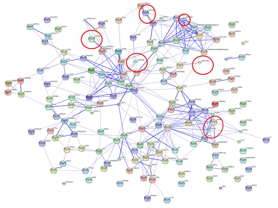 |
| Figure 1: Profile of one of the 6 samples under severe diet condition. |
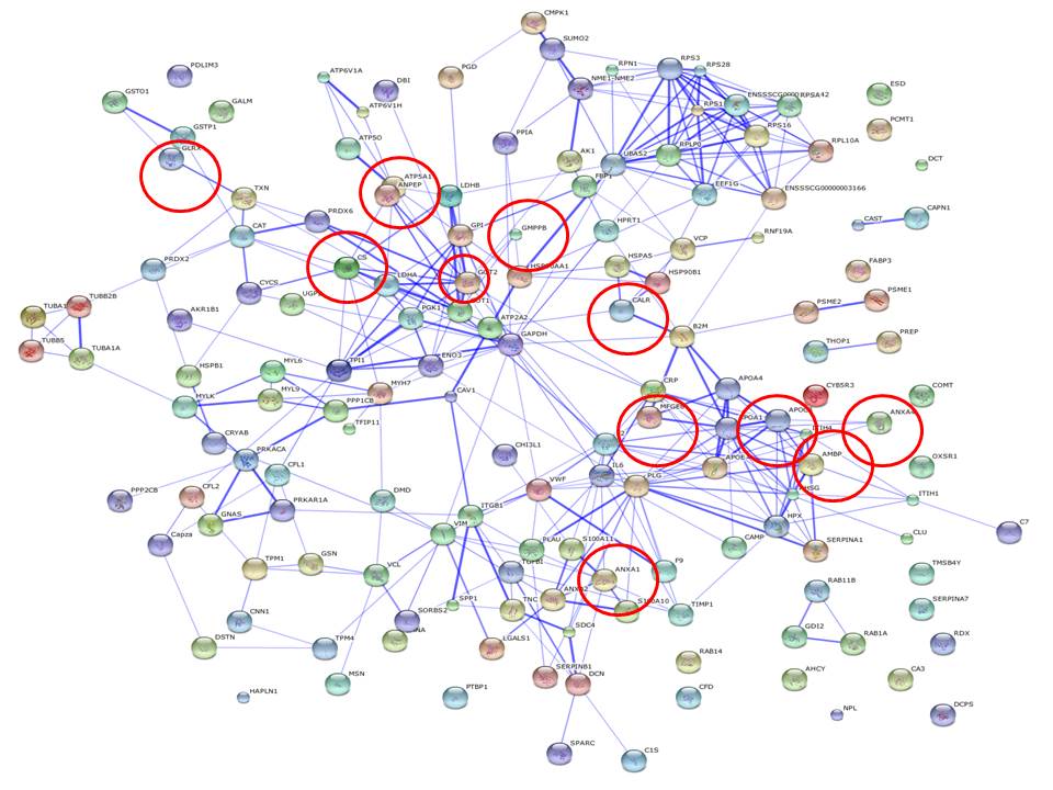 |
| Figure 2: Profile of another of the 6 samples under severe diet condition. |